Page:EB1911 - Volume 17.djvu/326

properties. The “magic circle of circles” (fig. 2) consists of eight annular rings and a central circle, each ring being divided into eight cells by radii drawn from the centre; there are therefore 65 cells. The number 12 is placed in the centre, and the consecutive numbers 13 to 75 are placed in the other cells. The properties of this figure include the following: (1) the sum of the eight numbers in any ring together with the central number 12 is 360, the number of degrees in a circle; (2) the sum of the eight numbers in any set of radial cells together with the central number is 360; (3) the sum of the numbers in any four adjoining cells, either annular, radial, or both radial and two annular, together with half the central number, is 180.

Construction of Magic Squares.—A square of 5 (fig. 3) has adjoining it one of the eight equal squares by which any square may be conceived to be surrounded, each of which has two sides resting on adjoining squares, while four have sides resting on the surrounded square, and four meet it only at its four angles. 1, 2, 3 are placed along the path of a knight in chess; 4, along the same path, would fall in a cell of the outer square, and is placed instead in the corresponding cell of the original square; 5 then falls within the square. a, b, c, d are placed diagonally in the square; but e enters the outer square, and is removed thence to the same cell of the square it had left. α, β, γ, δ, ε pursue another regular course; and the diagram shows how that course is recorded in the square they have twice left. Whichever of the eight surrounding squares may be entered, the corresponding cell of the central square is taken instead. The 1, 2, 3, . . ., a, b, c, . . ., α, β, γ, . . . are said to lie in “paths.”

Fig. 4.	Fig. 5.	Fig. 6.

Fig. 7.	Fig. 8.	Fig. 9.

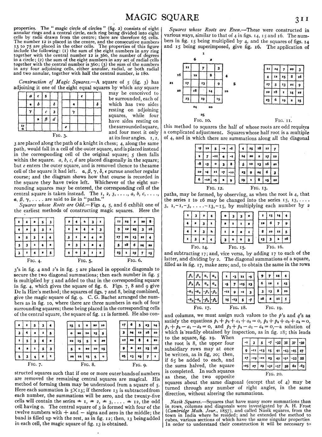
Squares whose Roots are Odd.—Figs 4, 5, and 6 exhibit one of the earliest methods of constructing magic squares. Here the 3’s in fig. 4 and 2’s in fig. 5 are placed in opposite diagonals to secure the two diagonal summations; then each number in fig. 5 is multiplied by 5 and added to that in the corresponding square in fig. 4, which gives the square of fig. 6. Figs. 7, 8 and 9 give De la Hire’s method; the squares of figs. 7 and 8, being combined, give the magic square of fig. 9. C. G. Bachet arranged the numbers as in fig. 10, where there are three numbers in each of four surrounding squares; these being placed in the corresponding cells of the central square, the square of fig. 11 is formed. He also constructed squares such that if one or more outer bands of numbers are removed the remaining central squares are magical. His method of forming them may be understood from a square of 5. Here each summation is 5×13; if therefore 13 is subtracted from each number, the summations will be zero, and the twenty-five cells will contain the series ± 1, ± 2, ± 3, . . . ± 12, the odd cell having 0. The central square of 3 is formed with four of the twelve numbers with + and − signs and zero in the middle; the band is filled up with the rest, as in fig. 12; then, 13 being added in each cell, the magic square of fig. 13 is obtained.

Fig. 10.	⁠Fig. 11.

Fig. 12.	Fig. 13.

Fig. 14.	Fig. 15.	Fig. 16.

Fig. 17.	Fig. 18.	Fig. 19.

Fig. 20.

Squares whose Roots are Even.—These were constructed in various ways, similar to that of 4 in figs. 14, 15 and 16. The numbers in fig. 15 being multiplied by 4, and the squares of figs. 14 and 15 being superimposed, give fig. 16. The application of this method to squares the half of whose roots are odd requires a complicated adjustment. Squares whose half root is a multiple of 4, and in which there are summations along all the diagonal paths, may be formed, by observing, as when the root is 4, that the series 1 to 16 may be changed into the series 15, 13, . . . 3, 1, −1, −3, . . . −13, −15, by multiplying each number by 2 and subtracting 17; and, vice versa, by adding 17 to each of the latter, and dividing by 2. The diagonal summations of a square, filled as in fig. 17, make zero; and, to obtain the same in the rows and columns, we must assign such values to the p’s and q’s as satisfy the equations p₁ + p₂ + a₁ + a₂ = 0, p₃ + p₄ + a₃ + a₄ = 0, p₁ + p₃ − a₁ − a₃ = 0, and p₂ + p₄ − a₂ − a₄ = 0,—a solution of which is readily obtained by inspection, as in fig. 18; this leads to the square, fig. 19. When the root is 8, the upper four subsidiary rows may at once be written, as in fig. 20; then, if 65 be added to each, and the sums halved, the square is completed. In such squares as these, the two opposite squares about the same diagonal (except that of 4) may be turned through any number of right angles, in the same direction, without altering the summations.

Nasik Squares.—Squares that have many more summations than in rows, columns and diagonals were investigated by A. H. Frost (Cambridge Math. Jour., 1857), and called Nasik squares, from the town in India where he resided; and he extended the method to cubes, various sections of which have the same singular properties. In order to understand their construction it will be necessary to